2.9 Animating Transformations

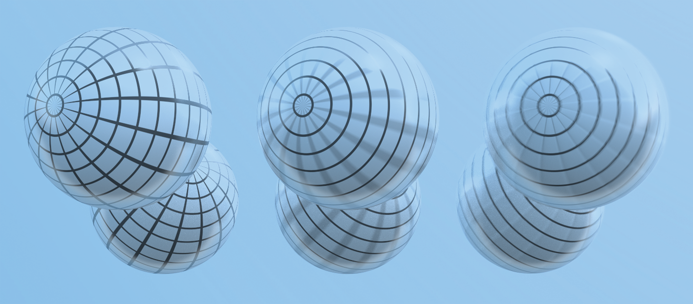
pbrt supports keyframe matrix animation for cameras and geometric primitives in the scene. Rather than just supplying a single transformation to place the corresponding object in the scene, the user may supply a number of keyframe transformations, each one associated with a particular point in time. This makes it possible for the camera to move and for objects in the scene to be moving during the time the simulated camera’s shutter is open. Figure 2.15 shows three spheres animated using keyframe matrix animation in pbrt.

In general, the problem of interpolating between keyframe matrices is under-defined. As one example, if we have a rotation about the axis of 181 degrees followed by another of 181 degrees, does this represent a small rotation of 2 degrees or a large rotation of degrees? For another example, consider two matrices where one is the identity and the other is a 180-degree rotation about the axis. There are an infinite number of ways to go from one orientation to the other.

Keyframe matrix interpolation is an important problem in computer animation, where a number of different approaches have been developed. Fortunately, the problem of matrix interpolation in a renderer is generally less challenging than it is for animation systems for two reasons.

First, in a renderer like pbrt, we generally have a keyframe matrix at the camera shutter open time and another at the shutter close time; we only need to interpolate between the two of them across the time of a single image. In animation systems, the matrices are generally available at a lower time frequency, so that there are many frames between pairs of keyframe matrices; as such, there’s more opportunity to notice shortcomings in the interpolation.

Second, in a physically based renderer, the longer the period of time over which we need to interpolate the pair of matrices, the longer the virtual camera shutter is open and the more motion blur there will be in the final image; the increased amount of motion blur often hides sins of the interpolation.

The most straightforward approach to interpolate transformations defined by keyframe matrices—directly interpolating the individual components of the matrices—is not a good one, as it will generally lead to unexpected and undesirable results. For example, if the transformations apply different rotations, then even if we have a rigid-body motion, the intermediate matrices may scale the object, which is clearly undesirable. (If the matrices have a full 180-degree rotation between them, the object may be scaled down to nothing at the middle of the interpolation!)

Figure 2.16 shows a sphere that rotates 90 degrees over the course of the frame; direct interpolation of matrix elements gives a less accurate result than the approach implemented in this section.

The approach used for transformation interpolation in pbrt is based on matrix decomposition—given an arbitrary transformation matrix , we decompose it into a concatenation of scale (), rotation (), and translation () transformations,

where each of those components is independently interpolated and then the composite interpolated matrix is found by multiplying the three interpolated matrices together.

Interpolation of translation and scale can be performed easily and accurately with linear interpolation of the components of their matrices; interpolating rotations is more difficult. Before describing the matrix decomposition implementation in pbrt, we will first introduce quaternions, an elegant representation of rotations that leads to effective methods for interpolating them.

2.9.1 Quaternions

Quaternions were originally invented by Sir William Rowan Hamilton in 1843 as a generalization of complex numbers. He determined that just as in two dimensions , where complex numbers could be defined as a sum of a real and an imaginary part , with , a generalization could be made to four dimensions, giving quaternions.

A quaternion is a four-tuple,

where , , and are defined ^† so that . Other important relationships between the components are that and . This implies that quaternion multiplication is generally not commutative.

A quaternion can be represented as a quadruple or as , where is an imaginary 3-vector and is the real part. We will use both representations interchangeably in this section.

An expression for the product of two arbitrary quaternions can be found by expanding their definition in terms of real and imaginary components:

Collecting terms and using identities among the components like those listed above (e.g., ), the result can be expressed concisely using vector cross and dot products:

There is a useful relationship between unit quaternions (quaternions whose components satisfy ) and the space of rotations in : specifically, a rotation of angle about a unit axis can be mapped to a unit quaternion , in which case the following quaternion product is equivalent to applying the rotation to a point expressed in homogeneous coordinate form:

Furthermore, the product of several rotation quaternions produces another quaternion that is equivalent to applying the rotations in sequence.

The implementation of the Quaternion class in pbrt is in the files core/quaternion.h and core/quaternion.cpp. The default constructor initializes a unit quaternion.

We use a Vector3f to represent the components of the quaternion; doing so lets us make use of various methods of Vector3f in the implementation of some of the methods below.

Addition and subtraction of quaternions is performed component-wise. This follows directly from the definition in Equation (2.4). For example,

Other arithmetic methods (subtraction, multiplication, and division by a scalar) are defined and implemented similarly and won’t be included here.

The inner product of two quaternions is implemented by its Dot() method, and a quaternion can be normalized by dividing by its length.

It’s useful to be able to compute the transformation matrix that represents the same rotation as a quaternion. In particular, after interpolating rotations with quaternions in the AnimatedTransform class, we’ll need to convert the interpolated rotation back to a transformation matrix to compute the final composite interpolated transformation.

To derive the rotation matrix for a quaternion, recall that the transformation of a point by a quaternion is given by . We want a matrix that performs the same transformation, so that . If we expand out the quaternion multiplication using Equation (2.5), simplify with the quaternion basis identities, collect terms, and represent the result in a matrix, we can determine that the following matrix represents the same transformation:

This computation is implemented in the method Quaternion::ToTransform(). We won’t include its implementation here since it’s a direct implementation of Equation (2.6).

Note that we could alternatively use the fact that a unit quaternion represents a rotation of angle around the unit axis to compute a rotation matrix. First we would compute the angle of rotation as , and then we’d use the previously defined Rotate() function, passing it the axis and the rotation angle . However, this alternative would be substantially less efficient, requiring multiple calls to trigonometric functions, while the approach implemented here only uses floating-point addition, subtraction, and multiplication.

It is also useful to be able to create a quaternion from a rotation matrix. For this purpose, Quaternion provides a constructor that takes a Transform. The appropriate quaternion can be computed by making use of relationships between elements of the rotation matrix in Equation (2.6) and quaternion components. For example, if we subtract the transpose of this matrix from itself, then the component of the resulting matrix has the value . Thus, given a particular instance of a rotation matrix with known values, it’s possible to use a number of relationships like this between the matrix values and the quaternion components to generate a system of equations that can be solved for the quaternion components.

We won’t include the details of the derivation or the actual implementation here in the text; for more information about how to derive this technique, including handling numerical robustness, see Shoemake (1991).

2.9.2 Quaternion Interpolation

The last quaternion function we will define, Slerp(), interpolates between two quaternions using spherical linear interpolation. Spherical linear interpolation gives constant speed motion along great circle arcs on the surface of a sphere and consequently has two desirable properties for interpolating rotations:

• The interpolated rotation path exhibits torque minimization: the path to get between two rotations is the shortest possible path in rotation space.
• The interpolation has constant angular velocity: the relationship between change in the animation parameter and the change in the resulting rotation is constant over the course of interpolation (in other words, the speed of interpolation is constant across the interpolation range).

See the “Further Reading” section at the end of the chapter for references that discuss more thoroughly what characteristics a good interpolated rotation should have.

Spherical linear interpolation for quaternions was originally presented by Shoemake (1985) as follows, where two quaternions and are given and is the parameter value to interpolate between them:

An intuitive way to understand Slerp() was presented by Blow (2004). As context, given the quaternions to interpolate between, and , denote by the angle between them. Then, given a parameter value , we’d like to find the intermediate quaternion that makes angle between it and , along the path from to .

An easy way to compute is to first compute an orthogonal coordinate system in the space of quaternions where one axis is and the other is a quaternion orthogonal to such that the two axes form a basis that spans and . Given such a coordinate system, we can compute rotations with respect to . (See Figure 2.17, which illustrates the concept in the 2D setting.) An orthogonal vector can be found by projecting onto and then subtracting the orthogonal projection from ; the remainder is guaranteed to be orthogonal to :

Given the coordinate system and a normalized , quaternions along the animation path are given by

The implementation of the Slerp() function checks to see if the two quaternions are nearly parallel, in which case it uses regular linear interpolation of quaternion components in order to avoid numerical instability. Otherwise, it computes an orthogonal quaternion qperp using Equation (2.7) and then computes the interpolated quaternion with Equation (2.8).

2.9.3 AnimatedTransform Implementation

Given the foundations of the quaternion infrastructure, we can now implement the AnimatedTransform class, which implements keyframe transformation interpolation in pbrt. Its constructor takes two transformations and the time values they are associated with.

As mentioned earlier, AnimatedTransform decomposes the given composite transformation matrices into scaling, rotation, and translation components. The decomposition is performed by the AnimatedTransform::Decompose() method.

Given the composite matrix for a transformation, information has been lost about any individual transformations that were composed to compute it. For example, given the matrix for the product of a translation and then a scale, an equal matrix could also be computed by first scaling and then translating (by different amounts). Thus, we need to choose a canonical sequence of transformations for the decomposition. For our needs here, the specific choice made isn’t significant. (It would be more important in an animation system that was decomposing composite transformations in order to make them editable by changing individual components, for example.)

We will handle only affine transformations here, which is what is needed for animating cameras and geometric primitives in a rendering system; perspective transformations aren’t generally relevant to animation of objects like these.

The transformation decomposition we will use is the following:

where is the given transformation, is a translation, is a rotation, and is a scale. is actually a generalized scale (Shoemake and Duff call it stretch) that represents a scale in some coordinate system, just not necessarily the current one. In any case, it can still be correctly interpolated with linear interpolation of its components. The Decompose() method computes the decomposition given a Matrix4x4.

Extracting the translation is easy; it can be found directly from the appropriate elements of the transformation matrix.

Since we are assuming an affine transformation (no projective components), after we remove the translation, what is left is the upper matrix that represents scaling and rotation together. This matrix is copied into a new matrix M for further processing.

Next we’d like to extract the pure rotation component of . We’ll use a technique called polar decomposition to do this. It can be shown that the polar decomposition of a matrix into rotation and scale can be computed by successively averaging with its inverse transpose

until convergence, at which point . (It’s easy to see that if is a pure rotation, then averaging it with its inverse transpose will leave it unchanged, since its inverse is equal to its transpose. The “Further Reading” section has more references that discuss why this series converges to the rotation component of the original transformation.) Shoemake and Duff (1992) proved that the resulting matrix is the closest orthogonal matrix to —a desirable property.

To compute this series, we iteratively apply Equation (2.10) until either the difference between successive terms is small or a fixed number of iterations have been performed. In practice, this series generally converges quickly.

Once we’ve extracted the rotation from , the scale is all that’s left. We would like to find the matrix that satisfies . Now that we know both and , we just solve for .

For every rotation matrix, there are two unit quaternions that correspond to the matrix that only differ in sign. If the dot product of the two rotations that we have extracted is negative, then a slerp between them won’t take the shortest path between the two corresponding rotations. Negating one of them (here the second was chosen arbitrarily) causes the shorter path to be taken instead.

The Interpolate() method computes the interpolated transformation matrix at a given time. The matrix is found by interpolating the previously extracted translation, rotation, and scale and then multiplying them together to get a composite matrix that represents the effect of the three transformations together.

If the given time value is outside the time range of the two transformations stored in the AnimatedTransform, then the transformation at the start time or end time is returned, as appropriate. The AnimatedTransform constructor also checks whether the two Transforms stored are the same; if so, then no interpolation is necessary either. All of the classes in pbrt that support animation always store an AnimatedTransform for their transformation, rather than storing either a Transform or AnimatedTransform as appropriate. This simplifies their implementations, though it does make it worthwhile to check for this case here and not unnecessarily do the work to interpolate between two equal transformations.

The dt variable stores the offset in the range from startTime to endTime; it is zero at startTime and one at endTime. Given dt, interpolation of the translation is trivial.

The rotation is interpolated between the start and end rotations using the Slerp() routine (Section 2.9.2).

Finally, the interpolated scale matrix is computed by interpolating the individual elements of the start and end scale matrices. Because the Matrix4x4 constructor sets the matrix to the identity matrix, we don’t need to initialize any of the other elements of scale.

Given the three interpolated parts, the product of their three transformation matrices gives us the final result.

AnimatedTransform also provides a number of methods that apply interpolated transformations directly, using the provided time for Point3fs and Vector3fs and Ray::time for Rays. These methods are more efficient than calling AnimatedTransform::Interpolate() and then using the returned matrix when there is no actual animation since a copy of the transformation matrix doesn’t need to be made in that case.

2.9.4 Bounding Moving Bounding Boxes

Given a Bounds3f that is transformed by an animated transformation, it’s useful to be able to compute a bounding box that encompasses all of its motion over the animation time period. For example, if we can bound the motion of an animated geometric primitive, then we can intersect rays with this bound to determine if the ray might intersect the object before incurring the cost of interpolating the primitive’s bound to the ray’s time to check that intersection. The AnimatedTransform::MotionBounds() method performs this computation, taking a bounding box and returning the bounding box of its motion over the AnimatedTransform’s time range.

There are two easy cases: first, if the keyframe matrices are equal, then we can arbitrarily apply only the starting transformation to compute the full bounds. Second, if the transformation only includes scaling and/or translation, then the bounding box that encompasses the bounding box’s transformed positions at both the start time and the end time bounds all of its motion. To see why this is so, consider the position of a transformed point as a function of time; we’ll denote this function of two matrices, a point, and a time by .

Since in this case the rotation component of the decomposition is the identity, then with our matrix decomposition we have

where the translation and scale are both written as functions of time. Assuming for simplicity that is a regular scale, we can find expressions for the components of . For example, for the component, we have:

where is the corresponding element of the scale matrix for , is the same scale matrix element for , and the translation matrix elements are similarly denoted by . (We chose for “delta” here since is already claimed for time.) As a linear function of , the extrema of this function are at the start and end times. The other coordinates and the case for a generalized scale follow similarly.

For the general case with animated rotations, the motion function may have extrema at points in the middle of the time range. We know of no simple way to find these points. Many renderers address this issue by sampling a large number of times in the time range, computing the interpolated transformation at each one, and taking the union of all of the corresponding transformed bounding boxes. Here, we will develop a more well-grounded method that lets us robustly compute these motion bounds.

We use a slightly simpler conservative bound that entails computing the motion of the eight corners of the bounding box individually and finding the union of those bounds.

For each bounding box corner , we need to find the extrema of over the animation time range. Recall from calculus that the extrema of a continuous function over some domain are either at the boundary points of the domain or at points where the function’s first derivative is zero. Thus, the overall bound is given by the union of the positions at the start and end of motion as well as the position at any extrema.

Figure 2.18 shows a plot of one coordinate of the motion function and its derivative for an interesting motion path of a point. Note that the maximum value of the function over the time range is reached at a point where the derivative has a zero.

To bound the motion of a single point, we start our derivation by following the approach used for the no-rotation case, expanding out the three , , and components of Equation (2.9) as functions of time and finding their product. We have:

The result is quite complex when expanded out, mostly due to the slerp and the conversion of the resulting quaternion to a matrix; a computer algebra system is a requirement for working with this function.

The derivative is also quite complex—in its full algebraic glory, over 2,000 operations are required to evaluate its value for a given pair of decomposed matrices, point and time. However, given specific transformation matrices and a specific point, is simplified substantially; we’ll denote the specialized function of alone as . Evaluating its derivative requires roughly 10 floating-point operations, a sine, and a cosine to evaluate for each coordinate:

where is the arc cosine of the dot product of the two quaternions and where the five coefficients are 3-vectors that depend on the two matrices and the position . This specialization works out well, since we will need to evaluate the function at many time values for a given point.

We now have two tasks: first, given a pair of keyframe matrices and a point , we first need to be able to efficiently compute the values of the coefficients . Then, given the relatively simple function defined by and , we need to find the zeros of Equation (2.12), which may represent the times at which motion extrema occur.

For the first task, we will first factor out the contributions to the coefficients that depend on the keyframe matrices from those that depend on the point , under the assumption that bounding boxes for multiple points’ motion will be computed for each pair of keyframe matrices (as is the case here). The result is fortunately quite simple—the vectors are linear functions of the point’s , , and components.

Thus, given the coefficients and a particular point we want to bound the motion of, we can efficiently compute the coefficients of the derivative function in Equation (2.12). The DerivativeTerm structure encapsulates these coefficients and this computation.

The attributes c1-c5 store derivative information corresponding to the five terms in Equation (2.12). The three array elements correspond to the three dimensions of space.

The fragment <<Compute terms of motion derivative function>> in the AnimatedTransform constructor, not included here, initializes these terms, via automatically generated code. Given that it requires a few thousand floating-point operations, doing this work once and amortizing over the multiple bounding box corners is helpful. The coefficients are more easily computed if we assume a canonical time range ; later, we’ll have to remap the values of zeros of the motion function to the actual shutter time range.

Given the coefficients based on the keyframe matrices, BoundPointMotion() computes a robust bound of the motion of p.

The IntervalFindZeros() function, to be introduced shortly, numerically finds zeros of Equation (2.12). Up to four are possible.

The zeros are found over , so we need to interpolate within the time range before calling the method to transform the point at the corresponding time. Note also that the extremum is only at one of the , , and  dimensions, and so the bounds only need to be updated in that one dimension. For convenience, here we just use the Union() function, which considers all dimensions, even though two could be ignored.

Finding zeros of the motion derivative function, Equation (2.12), can’t be done algebraically; numerical methods are necessary. Fortunately, the function is well behaved—it’s fairly smooth and has a limited number of zeros. (Recall the plot in Figure 2.18, which was an unusually complex representative.)

While we could use a bisection-based search or Newton’s method, we’d risk missing zeros when the function only briefly crosses the axis. Therefore, we’ll use interval arithmetic, an extension of arithmetic that gives insight about the behavior of functions over ranges of values, which makes it possible to robustly find zeros of functions.

To understand the basic idea of interval arithmetic, consider, for example, the function . If we have an interval of values , then we can see that over the interval, the range of is the interval . In other words .

More generally, all of the basic operations of arithmetic have interval extensions that describe how they operate on intervals. For example, given two intervals and ,

In other words, if we add together two values where one is in the range and the second is in , then the result must be in the range .

Interval arithmetic has the important property that the intervals that it gives are conservative. In particular, if and if , then we know for sure that no value in causes to be negative. In the following, we will show how to compute Equation (2.12) over intervals and will take advantage of the conservative bounds of computed intervals to efficiently find small intervals with zero crossings where regular root finding methods can be reliably used.

First we will define an Interval class that represents intervals of real numbers.

An interval can be initialized with a single value, representing a single point on the real number line, or with two values that specify an interval with non-zero width.

The class also provides overloads for the basic arithmetic operations. Note that for subtraction, the high value of the second interval is subtracted from the low value of the first. ^†

For multiplication, which sides of each interval determine the minimum and maximum values of the result interval depend on the signs of the respective values. Multiplying the various possibilities and taking the overall minimum and maximum is easier than working through which ones to use and multiplying these.

We have also implemented Sin() and Cos() functions for Intervals. The implementations assume that the given interval is in , which is the case for our use of these functions. Here we only include the implementation of Sin(); Cos() is quite similar in basic structure.

Given the interval machinery, we can now implement the IntervalFindZeros() function, which finds the values of any zero crossings of Equation (2.12) over the given interval tInterval.

The function starts by computing the interval range over tInterval. If the range doesn’t span zero, then there are no zeros of the function over tInterval and the function can return.

If the interval range does span zero, then there may be one or more zeros in the interval tInterval, but it’s also possible that there actually aren’t any, since the interval bounds are conservative but not as tight as possible. The function splits tInterval into two parts and recursively checks the two sub-intervals. Reducing the size of the interval domain generally reduces the extent of the interval range, which may allow us to determine that there are no zeros in one or both of the new intervals.

Once we have a narrow interval where the interval value of the motion derivative function spans zero, the implementation switches to a few iterations of Newton’s method to find the zero, starting at the midpoint of the interval. Newton’s method requires the derivative of the function; since we’re finding zeros of the motion derivative function, this is the second derivative of Equation (2.11):

Note that if there were multiple zeros of the function in tInterval when Newton’s method is used, then we will only find one of them here. However, because the interval is quite small at this point, the impact of this error should be minimal. In any case, we haven’t found this issue to be a problem in practice.