3.7 Curves

While triangles can be used to represent thin shapes for modeling fine geometry like hair, fur, or fields of grass, it’s worthwhile to have a specialized Shape in order to more efficiently render these sorts of objects, since many individual instances of them are often present. The Curve shape, introduced in this section, represents thin geometry modeled with cubic Bézier splines, which are defined by four control points, , , , and . The Bézier spline passes through the first and last control points; intermediate points are given by the polynomial

(See Figure 3.15.) Given a curve specified in another cubic basis, such as a Hermite spline, it’s easy enough to convert to Bézier basis, so the implementation here leaves that burden on the user. This functionality could be easily added if it was frequently needed.

The Curve shape is defined by a 1D Bézier curve along with a width that is linearly interpolated from starting and ending widths along its extent. Together, these define a flat 2D surface (Figure 3.16). ^† It’s possible to directly intersect rays with this representation without tessellating it, which in turn makes it possible to efficiently render smooth curves without using too much storage.

Figure 3.17 shows a bunny model with fur modeled with over one million Curves.

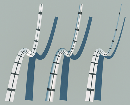
There are three types of curves that the Curve shape can represent, shown in Figure 3.18.

• Flat: Curves with this representation are always oriented to face the ray being intersected with them; they are useful for modeling fine swept cylindrical shapes like hair or fur.
• Cylinder: For curves that span a few pixels on the screen (like spaghetti seen from not too far away), the Curve shape can compute a shading normal that makes the curve appear to actually be a cylinder.
• Ribbon: This variant is useful for modeling shapes that don’t actually have a cylindrical cross section (such as a blade of grass).

The CurveType enumerant records which of them a given Curve instance models.

The flat and cylinder curve variants are intended to be used as convenient approximations of deformed cylinders. It should be noted that intersections found with respect to them do not correspond to a physically realizable 3D shape, which can potentially lead to minor inconsistencies when taking a scene with true cylinders as a reference.

Given a curve specified in a pbrt scene description file, it can be worthwhile to split it into a few segments, each covering part of the parametric range of the curve. (One reason for doing so is that axis-aligned bounding boxes don’t tightly bound wiggly curves, but subdividing Bézier splines makes them less wiggly—the variation diminishing property of polynomial splines.) Therefore, the Curve constructor takes both a parametric range of values, , as well as a pointer to a CurveCommon structure, which stores the control points and other information about the curve that is shared across curve segments. In this way, the memory footprint for individual curve segments is minimized, which makes it easier to keep many of them in memory.

The CurveCommon constructor mostly just initializes member variables with values passed into it for the control points, the curve width, etc. The control points provided to it should be in the curve’s object space.

For Ribbon curves, CurveCommon stores a surface normal to orient the curve at each endpoint. The constructor precomputes the angle between the two normal vectors and one over the sine of this angle; these values will be useful when computing the orientation of the curve at arbitrary points along its extent.

Bounding boxes of Curves can be computed by taking advantage of the convex hull property, a property of Bézier curves that says that they must lie within the convex hull of their control points. Therefore, the bounding box of the control points gives a conservative bound of the underlying curve. The ObjectBound() method first computes a bounding box of the control points of the 1D Bézier segment to bound the spline along the center of the curve. These bounds are then expanded by half the maximum width the curve takes on over its parametric extent to get the 3D bounds of the Shape that the Curve represents.

The CurveCommon class stores the control points for the full curve, but Curve instances generally need the four control points that represent the Bézier curve for its extent. These control points are computed using a technique called blossoming. The blossom of a cubic Bézier spline is defined by three stages of linear interpolation, starting with the original control points:

The blossom gives the curve’s value at position . (To verify this for yourself, expand Equation (3.4) using , simplify, and compare to Equation (3.3).)

BlossomBezier() implements this computation.

The four control points for the curve segment over the range to are given by the blossoms:

(Figure 3.19).

Given this machinery, it’s straightforward to compute the four control points for the curve segment that a Curve is responsible for.

The Curve intersection algorithm is based on discarding curve segments as soon as it can be determined that the ray definitely doesn’t intersect them and otherwise recursively splitting the curve in half to create two smaller segments that are then tested. Eventually, the curve is linearly approximated for an efficient intersection test. After some preparation, the recursiveIntersect() call starts this process with the full segment that the Curve represents.

Like the ray–triangle intersection algorithm from Section 3.6.2, the ray–curve intersection test is based on transforming the curve to a coordinate system with the ray’s origin at the origin of the coordinate system and the ray’s direction aligned to be along the axis. Performing this transformation at the start greatly reduces the number of operations that must be performed for intersection tests.

For the Curve shape, we’ll need an explicit representation of the transformation, so the LookAt() function is used to generate it here. The origin is the ray’s origin, the “look at” point is a point offset from the origin along the ray’s direction, and the “up” direction is an arbitrary direction orthogonal to the ray direction.

The maximum number of times to subdivide the curve is computed so that the maximum distance from the eventual linearized curve at the finest refinement level is bounded to be less than a small fixed distance. We won’t go into the details of this computation, which is implemented in the fragment <<Compute refinement depth for curve, maxDepth>>.

The recursiveIntersect() method then tests whether the given ray intersects the given curve segment over the given parametric range .

The method starts by checking to see if the ray intersects the curve segment’s bounding box; if it doesn’t, no intersection is possible and it can return immediately.

Along the lines of the implementation in Curve::ObjectBound(), a conservative bounding box for the segment can be found by taking the bounds of the curve’s control points and expanding by half of the maximum width of the curve over the range being considered.

Because the ray’s origin is at and its direction is aligned with the axis in the intersection space, its bounding box only includes the origin in and (Figure 3.20); its extent is given by the range that its parametric extent covers.

If the ray does intersect the curve’s bounding box and the recursive splitting hasn’t bottomed out, then the curve is split in half along the parametric range. SubdivideBezier() computes seven control points: the first four correspond to the control points for the first half of the split curve, and the last four (starting with the last control point of the first half) correspond to the control points for the second half. Two calls to recursiveIntersect() test the two sub-segments.

While we could use the BlossomBezier() function to compute the control points of the subdivided curves, they can be more efficiently computed by taking advantage of the fact that we’re always splitting the curve exactly in the middle of its parametric extent. This computation is implemented in the SubdivideBezier() function; the seven control points it computes correspond to using , , , , , , and as blossoms in Equation (3.4).

After a number of subdivisions, an intersection test is performed. Parts of this test are made more efficient by using a linear approximation of the curve; the variation diminishing property allows us to make this approximation without introducing too much error.

It’s important that the intersection test only accept intersections that are on the Curve’s surface for the segment currently under consideration. Therefore, the first step of the intersection test is to compute edge functions for lines perpendicular to the curve starting point and ending point and to classify the potential intersection point against them (Figure 3.21).

Projecting the curve control points into the ray coordinate system makes this test more efficient for two reasons. First, because the ray’s direction is oriented with the axis, the problem is reduced to a 2D test in and . Second, because the ray origin is at the origin of the coordinate system, the point we need to classify is , which simplifies evaluating the edge function, just like the ray–triangle intersection test.

Edge functions were introduced for ray–triangle intersection tests in Equation (3.1); see also Figure 3.14. To define the edge function, we need any two points on the line perpendicular to the curve going through starting point. The first control point, , is a fine choice for the first point. For the second one, we’ll compute the vector perpendicular to the curve’s tangent and add that offset to the control point.

Differentiation of Equation (3.3) shows that the tangent to the curve at the first control point is . The scaling factor doesn’t matter here, so we’ll use here. Computing the vector perpendicular to the tangent is easy in 2D: it’s just necessary to swap the and coordinates and negate one of them. (To see why this works, consider the dot product . Because the cosine of the angle between the two vectors is zero, they must be perpendicular.) Thus, the second point on the edge is

Substituting these two points into the definition of the edge function, Equation (3.1), and simplifying gives

Finally, substituting gives the final expression to test:

The <<Test sample point against tangent perpendicular at curve end>> fragment, not included here, does the corresponding test at the end of the curve.

The next part of the test is to determine the value along the curve segment where the point is closest to the curve. This will be the intersection point, if it’s no farther than the curve’s width away from the center at that point. Determining this distance for a cubic Bézier curve is not efficient, so instead this intersection approach approximates the curve with a linear segment to compute this value.

We’ll linearly approximate the Bézier curve with a line segment from its starting point to its end point that is parameterized by . In this case, the position is at and at (Figure 3.22). Our task now is to compute the value of along the line corresponding to the point on the line that is closest to the point . The key insight to apply is that at , the vector from the corresponding point on the line to will be perpendicular to the line (Figure 3.23 (a)).

Equation (2.1) gives us a relationship between the dot product of two vectors, their lengths, and the cosine of the angle between them. In particular, it shows us how to compute the cosine of the angle between the vector from to and the vector from to :

Because the vector from to is perpendicular to the line (Figure 3.23(b)), then we can compute the distance along the line from to as

Finally, the parametric offset along the line is the ratio of to the line’s length,

The computation of the value of is in turn slightly simplified from the fact that in the intersection coordinate system.

The parametric coordinate of the (presumed) closest point on the Bézier curve to the candidate intersection point is computed by linearly interpolating along the range of the segment. Given this value, the width of the curve at that point can be computed.

For Ribbon curves, the curve is not always oriented to face the ray. Rather, its orientation is interpolated between two surface normals given at each endpoint. Here, spherical linear interpolation is used to interpolate the normal at (recall Section 2.9.2). The curve’s width is then scaled by the cosine of the angle between the normalized ray direction and the ribbon’s orientation so that it reflects the visible width of the curve from the given direction.

To finally classify the potential intersection as a hit or miss, the Bézier curve must still be evaluated at using the EvalBezier() function. (Because the control points cp represent the curve segment currently under consideration, it’s important to use rather than in the function call, however, since is in the range .) The derivative of the curve at this point will be useful shortly, so it’s recorded now.

We’d like to test whether the distance from to this point on the curve pc is less than half the curve’s width. Because , we can equivalently test whether the distance from pc to the origin is less than half the width or, equivalently, whether the squared distance is less than one quarter the width squared. If this test passes, the last thing to check is if the intersection point is in the ray’s parametric range.

EvalBezier() computes the blossom to evaluate a point on a Bézier spline. It optionally also returns the derivative of the curve at the point.

If the earlier tests have all passed, we have found a valid intersection, and the coordinate of the intersection point can now be computed. The curve’s coordinate ranges from 0 to 1, taking on the value at the center of the curve; here, we classify the intersection point, , with respect to an edge function going through the point on the curve pc and a point along its derivative to determine which side of the center the intersection point is on and in turn how to compute .

Finally, the partial derivatives are computed, and the SurfaceInteraction for the intersection can be initialized.

The partial derivative comes directly from the derivative of the underlying Bézier curve. The second partial derivative, , is computed in different ways based on the type of the curve. For ribbons, we have and the surface normal, and so must be the vector such that and has length equal to the curve’s width.

For flat and cylinder curves, we transform to the intersection coordinate system. For flat curves, we know that lies in the plane, is perpendicular to , and has length equal to hitWidth. We can find the 2D perpendicular vector using the same approach as was used earlier for the perpendicular curve segment boundary edges.

The vector for cylinder curves is rotated around the dpduPlane axis so that its appearance resembles a cylindrical cross-section.

The Curve::Area() method, not included here, first approximates the curve length by the length of its control hull. It then multiplies this length by the average curve width over its extent to approximate the overall surface area.